1. Neural Network Fundamentals
1.1 Introduction to Artificial Neural Networks
Artificial Neural Networks (ANNs) are mathematical functions that can produce approximations of real values, discrete values (integer or categorical), or vectors of values. They're built out of a densely interconnected set of units where each unit takes real-valued inputs (possibly the outputs of other units) and produces a single real-valued output (which may become the input to other units).
ANNs are particularly useful for:
- Pattern recognition
- Classification tasks
- Function approximation
- Data processing
- Robotics
- Control systems
1.2 Biological Inspiration
ANNs were inspired by biological neurons and their connectionist nature in the human brain:
- The human brain contains approximately neurons and synapses, with a cycle time of seconds
- Biological neurons have dendrites that receive signals, a cell body (soma) that processes them, and an axon that transmits signals to other neurons
- Synapses are junctions that allow signal transmission between neurons and may be excitatory or inhibitory
- When inputs reach a threshold, an action potential (electrical pulse) is sent along the axon to outputs
While inspired by biological neurons, ANNs have many simplifications and inconsistencies:
- ANNs output a single value, whereas biological neurons output complex time series of spikes
- ANNs use simplified mathematical models rather than detailed biochemical processes
There have been two main directions in neural network research:
- Trying to simulate how the human brain works (modeling the process)
- Producing machine learning methodologies (modeling the outcome without mimicking the process)
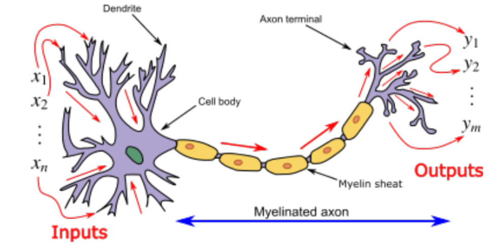
Showing applications of neural networks
1.3 Basic Components and Structure
The fundamental building block of an ANN is a neuron (also called a node or unit). Neural network nodes have:
- Input edges, each with an associated weight
- Output edges (with weights)
- An activation level (function of inputs)
- A transfer/activation function
The key components and their relationships are:
Weights: Connection strengths between neurons that can be positive or negative and may change during learning
Input function: Typically calculated as the weighted sum of inputs:
Where:- is the input to neuron
- is the weight from input to neuron
- is the value of input
- is the number of inputs
Activation function: A non-linear function applied to the input sum:
Network structure: ANNs typically have:
- An input layer that receives external data
- One or more hidden layers for processing
- An output layer that produces the final result
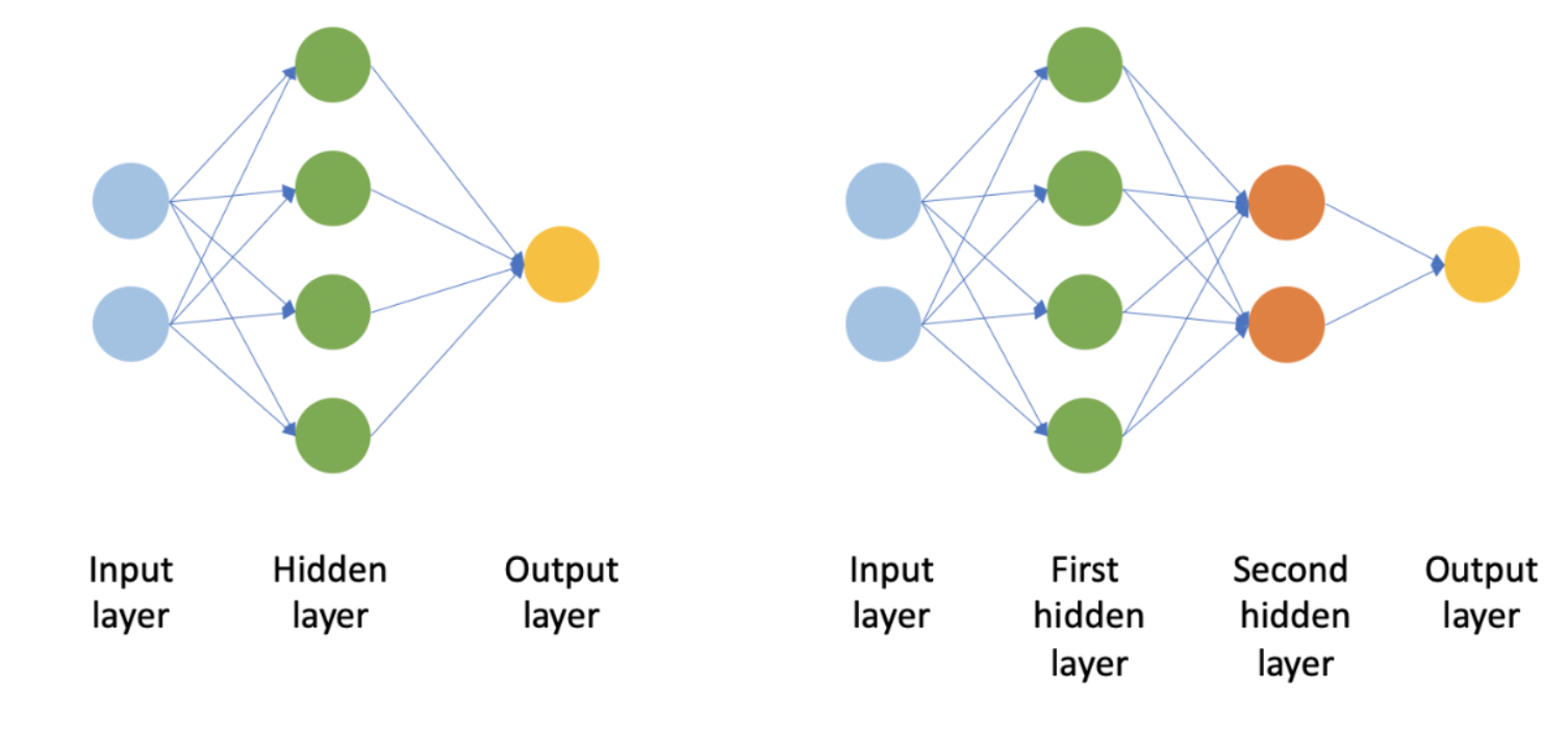
Showing a feedforward network structure
- Bias: Most neurons include a bias term that allows shifting the activation function:
Where:
- is the bias term (often implemented by setting )
Example of basic computation in a neuron:
Let's consider a neuron with 3 inputs: , , With weights: , , , and bias
The input sum would be:
If using a sigmoid activation function
the output would be:
2. Perceptrons and Single-Layer Networks
2.1 Perceptron Structure
A perceptron is the simplest type of artificial neural network, consisting of a single neuron. It was one of the earliest models of neural networks developed in the 1950s.
The perceptron takes several binary inputs and produces a single binary output based on a weighted sum of the inputs. The structure includes:
- A set of inputs ()
- Associated weights ()
- A bias weight () with constant input
- A threshold (th) that determines when the perceptron activates
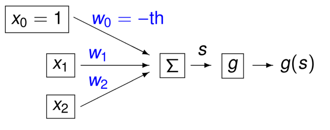
Showing perceptron structure with inputs, weights, and output
The perceptron computes the weighted sum of inputs plus the bias term:
Where:
- is the weighted sum
- are the weights
- are the inputs
- is often represented as a bias weight with
This sum is then passed through a threshold function to produce the output:
2.2 Transfer/Threshold Functions
The transfer function (also called threshold or activation function) determines the output of the perceptron based on the weighted sum of inputs. Common transfer functions include:
Sign Function
The output is either 1 or -1 depending on the input. This can be used for binary classification where:
- If the total input is positive, the sample is assigned to class 1
- If the total input is negative, the sample is assigned to class -1
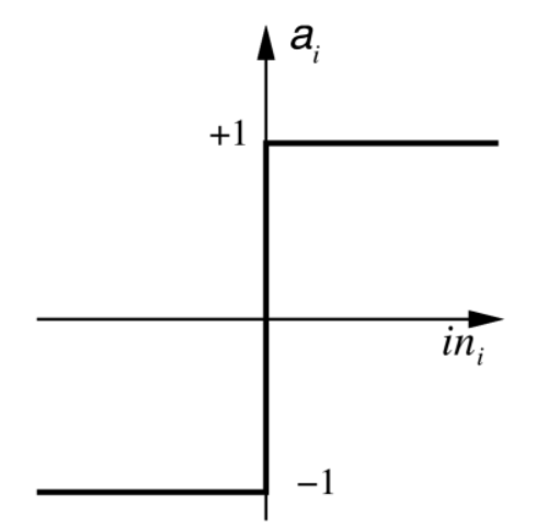
The continuous version of the sign function is the hyperbolid tangent function
Step Function
Where:
- is a threshold value (often 0).
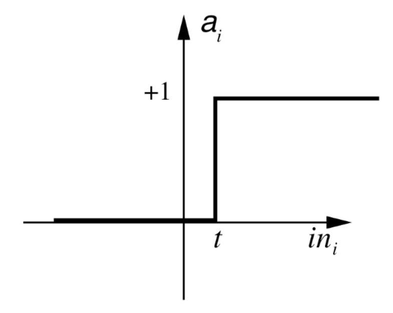
The continuous version of the sign function is the sigmoid function
Sigmoid Function
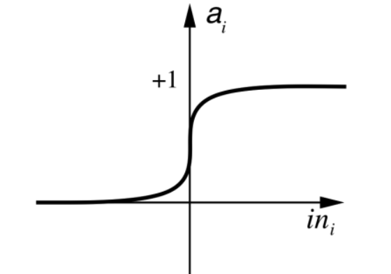
Sigmoid function
The sigmoid function has several advantages:
- Maps any real-valued number into the range (0, 1) - useful for representing probability
- Nearly linear around 0 but flattens toward the ends - squashes outlier values toward 0 or 1
- Differentiable, which is important for training algorithms
With the sigmoid function, we have the partial derivative:
This derivative is key for training algorithms like backpropagation.
Hyperbolic Tangent () Function
Similar to the sigmoid, but outputs values in the range instead of .
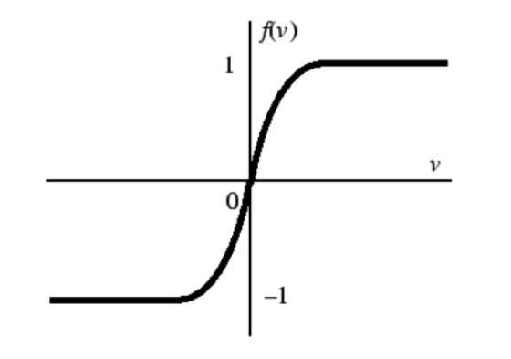
Hyperbolid tangent function
2.3 Linearly Separable Functions
A linearly separable function is one where the input space can be divided by a hyperplane (a line in 2D, a plane in 3D, etc.) such that all inputs on one side of the hyperplane are in one class, and all inputs on the other side are in the other class.
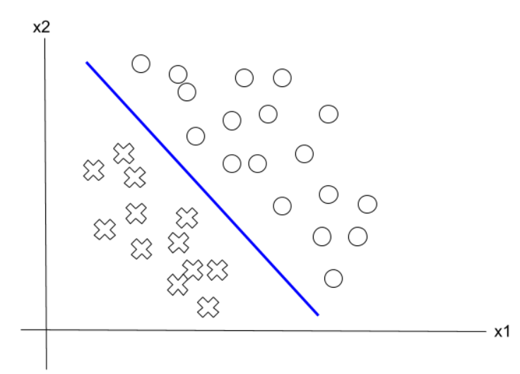
A single perceptron can only compute linearly separable functions. This is both a strength (simplicity) and a limitation (can't solve more complex problems).
For a perceptron with weights , the decision boundary is defined by:
Examples of linearly separable functions that a perceptron can compute:
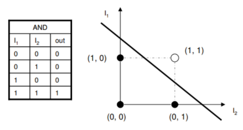
AND Function
With weights and bias :
| (Step function) | |||
|---|---|---|---|
| 0 | 0 | 0 | |
| 0 | 1 | 0 | |
| 1 | 0 | 0 | |
| 1 | 1 | 1 |
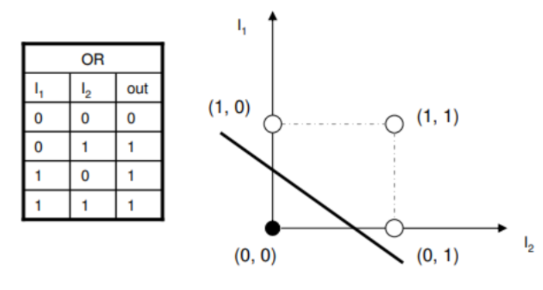
OR Function
With weights and bias :
| (Step function) | |||
|---|---|---|---|
| 0 | 0 | 0 | |
| 0 | 1 | 1 | |
| 1 | 0 | 1 | |
| 1 | 1 | 1 |
Example
If we have the following 2-dimensional examples from two classes:
- Class A: [-2 -2]; [2 2]
- Class B: [3 3]
We can use a perceptron to distinguish between them because the data is linearly separable.
However, for data that isn't linearly separable (like the XOR function), a single perceptron cannot correctly classify all points.
2.4 Training Methods
The weights of a perceptron must be adjusted to solve a particular problem. There are three primary methods for training single-layer networks:
2.4.1 Error Correction Method / Perceptron Learning Rule
The error correction method/perceptron learning rule adjusts weights based on the error between the desired output and the actual output.
Algorithm:
- Begin with random weights
- Repeat until stopping condition:
- For each training example, update each weight by:
- For each training example, update each weight by:
Where:
- is the learning rate (controls how quickly weights change)
- is the target output (desired value)
- is the actual output from the network
- is the input value
Intuition behind the update rule:
- If , no update is needed
- If (perceptron outputs -1 when target is 1), increase weights associated with positive inputs
- If (perceptron outputs 1 when target is -1), decrease weights associated with positive inputs
Convergence Theorem: If the boundary between classes is linear, and the learning rate is small enough, the error correction method will find it within a finite number of steps, classifying all training examples correctly.
Example:
Let's consider a simple perceptron with two input features plus bias, using the error correction method with learning rate and step function .
Initial weights: (bias), ,
Example 1: No update needed
Input: , , desired output
Calculate weighted sum:
Apply activation function: (since )
Since , no update is needed.
Example 2: Update needed
Input: , , desired output
Calculate weighted sum:
Apply activation function: (since )
Since and , update is needed:
Updated weights: , ,
2.4.2 Delta Rule / Widrow-Hoff Learning Rule / Least Mean Square Rule
The delta rule/Widrow-Hoff learning rule/least mean square rule is based on gradient descent and minimizes the squared error between the target output and the actual output.
The key difference from the error correction method is that the delta rule compares the target with the weighted sum directly, not with the thresholded output .
Error function:
Where:
- is the number of training instances
- is the target value for instance
- is the weighted sum output for instance
This is effectively linear regression, as we're trying to find the weights that minimize the squared difference between the target and the weighted sum.
Weight update rule:
After calculating the partial derivative, this simplifies to:
Training approaches:
- Batch gradient descent: Sum errors over all training examples before adjusting weights
- Stochastic gradient descent: Adjust weights after each example
Example:
Let's consider a simple perceptron with two input features plus bias, using the delta rule with learning rate .
Initial weights: (bias), ,
Example 1: Delta Rule Update
Input: , , desired output
Calculate weighted sum:
For delta rule, we update whenever , so we need an update:
Updated weights: , ,
Example 2: Another Delta Rule Update
Input: , , desired output
Calculate weighted sum:
Updated weights: , ,
2.4.3 Generalised Delta Rule
The generalised delta rule extends the delta rule by incorporating the transfer function into the error calculation.
Error function:
Where is the output after applying the transfer function.
Weight update rule: For a differentiable transfer function like sigmoid:
Where:
- is the derivative of the sigmoid function
When using the sigmoid function:
- varies from 0 to 0.25
- It equals 0 when is 0 or 1
- It reaches maximum value of 0.25 when is 0.5
Example with sigmoid transfer function:
Let's use the generalised delta rule with sigmoid transfer function . The update rule is:
Initial weights: (bias), , Learning rate:
Generalised Delta Rule Example
Input: , , desired output
Calculate weighted sum:
Apply sigmoid function:
Calculate derivative term:
Update the weights:
Updated weights: , ,
2.5 Limitations of Single-Layer Networks
The fundamental limitation of single-layer networks is that they can only solve linearly separable problems. This was proven mathematically by Minsky and Papert in their 1969 book "Perceptrons."
XOR Problem: The classic example of this limitation is the XOR (exclusive OR) function:
| Input A | Input B | XOR Output |
|---|---|---|
| 0 | 0 | 0 |
| 0 | 1 | 1 |
| 1 | 0 | 1 |
| 1 | 1 | 0 |
No single straight line can separate the points (0,0) and (1,1) from (0,1) and (1,0) in the input space.
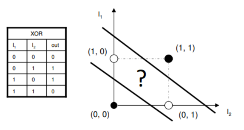
Showing XOR problem not being linearly separable
However, XOR can be represented as a combination of simpler functions:
Or more simply:
This suggests a solution: multi-layer networks where each layer can compute a different linearly separable function, and their combination can represent more complex, non-linear functions.
Possible solutions to overcome single-layer limitations:
- Use multiple layers of perceptrons
- Transform the input space using non-linear features
- Use more powerful classifiers
The discovery of effective training algorithms for multi-layer networks (like backpropagation) was a major breakthrough that revitalized the field of neural networks after the initial discouragement from the perceptron's limitations.
3. Multi-Layer Networks
3.1 Structure and Function
Multi-layer networks (also called multi-layer perceptrons or MLPs) consist of one input layer, one output layer, and one or more hidden layers of processing units. This structure allows them to overcome the limitations of single-layer networks.

Showing the layered structure of a feedforward network
A feedforward network has a structured architecture where:
- Each layer consists of units (neurons) that receive input from the layer below
- Units send their output to units in the layer directly above
- There are no connections within a layer
- Information flows in one direction (forward)
The mathematical representation of how data passes through a multi-layer network:
Input to hidden layer (for a network with input nodes and hidden nodes):
Where:
- is the output of the -th hidden neuron
- is the -th input
- is the weight from input to hidden neuron
- is the activation function
- is the weighted sum input to hidden neuron
Hidden to output layer (for hidden nodes and an output layer):
Where:
- is the output of the -th output neuron
- is the output from the -th hidden neuron
- is the weight from hidden neuron to output neuron
Including bias terms (common in practice):
Where and are bias terms for the respective neurons
Key components of multi-layer networks:
- Hidden layers produce hidden values that are non-linear functions of the inputs
- Non-linear activation functions are applied at each layer
- Weights are applied at each layer and adjusted during learning
- Output layer produces the final result, often using a non-linear threshold function
3.2 Representational Power
The power of multi-layer networks comes from their ability to represent complex functions that single-layer networks cannot.
Universal Function Approximator Theorem: A feed-forward neural network with at least one hidden layer (and a sufficient number of hidden units) can approximate almost any continuous function.
This theorem is fundamental to understanding why neural networks are such powerful models. It states that:
- Given enough hidden units, a two-layer network can approximate any continuous function to arbitrary precision
- The approximation improves as more hidden units are added
- This applies to networks using a variety of activation functions (sigmoid, tanh, etc.)
Practical implications:
- Multi-layer networks can learn highly complex, non-linear mappings from inputs to outputs
- They can represent decision boundaries that aren't possible with single-layer networks
- The complexity of functions they can represent increases with:
- Number of layers (depth)
- Number of neurons per layer (width)
Example: XOR Problem Solution A multi-layer network can solve the XOR problem that single-layer perceptrons cannot:
- First hidden layer: Compute AND and OR functions
Second layer: Combine these to form XOR
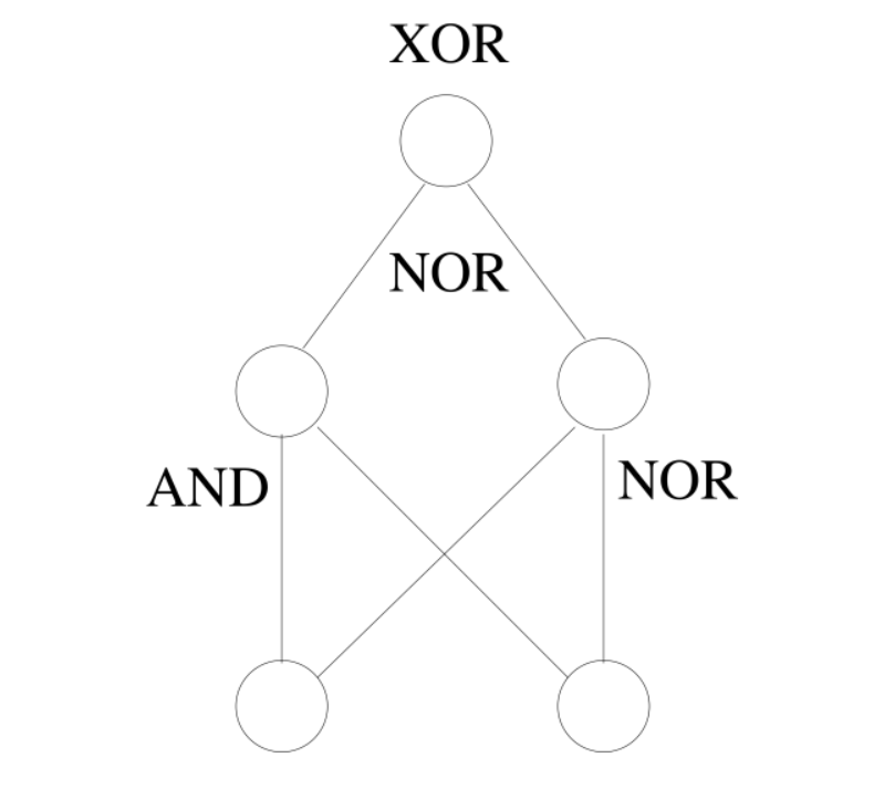 This demonstrates how complex functions can be built from simpler ones through layering.
3.3 Non-linearity
Non-linearity is crucial in neural networks because without it, a multi-layer network would be mathematically equivalent to a single-layer network.
Why non-linearity matters:
- Linear functions composed with linear functions remain linear
- Non-linear activation functions enable networks to learn complex patterns
- They allow the creation of complex decision boundaries
Building complex boundaries from simple components:
A multi-layer network with non-linear activation functions can create increasingly complex decision boundaries:
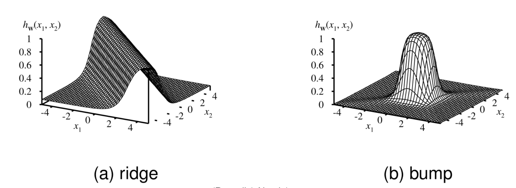
Showing ridge and bump patterns created by combining sigmoid functions
The diagram shows:
- (a) A ridge formed by combining two opposite-facing soft threshold functions
- (b) A bump created by combining two ridges
This visual representation demonstrates how neural networks stack simple non-linear functions to create complex patterns in the decision space.
Mathematical example of non-linear construction:
Consider a 2-dimensional input space. With appropriate weights, hidden units can create:
- Linear boundaries (like lines in 2D space)
- These linear boundaries can be combined through non-linear functions to create:
- Half-planes
- Convex regions
- Arbitrary regions through unions and intersections
Non-linear activation in practice:
Without non-linearity:
- A multi-layer network of linear functions creates a piece-wise linear boundary
- A multi-layer linear network is mathematically equivalent to a single-layer linear network
With non-linearity:
- Each layer transforms the data in a way that makes patterns more separable
- Complex, smooth decision boundaries become possible
- The network can approximate any continuous function (as per the Universal Approximator Theorem)
This non-linear capability is what makes neural networks so powerful for complex pattern recognition tasks that linear models cannot handle.
4. Backpropagation
4.1 Gradient Descent in Neural Networks
Backpropagation is the classic algorithm used to train multi-layer neural networks. It works by propagating the error backwards through the network to adjust weights using gradient descent.
The training process involves:
- Forward pass to calculate outputs and error
- Backward pass to adjust weights proportionally to their contribution to the error
- Iterating this process until convergence
The error function for a neural network with multiple outputs is typically defined as:
Where:
- is the total error
- is the target/desired output for output unit
- is the actual output from output unit
- The sum is over all output units
For gradient descent, we need to find how the error changes with respect to each weight in the network:
Where:
- is the weight update
- is the learning rate
- is the partial derivative of the error with respect to the weight
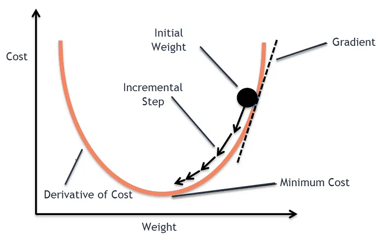
The backpropagation algorithm efficiently computes these derivatives by applying the chain rule of calculus, working backwards from the output layer to the input layer.
4.2 Weight Updates
4.2.1 Hidden to Output Layer
To update weights between the hidden and output layers, we need to determine how much each weight contributes to the error.
For a weight connecting hidden unit to output unit :
Where:
- is the output of unit
- is the weighted sum input to unit :
- is the output from hidden unit
Breaking down each term:
Error gradient with respect to output:
Output gradient with respect to weighted sum (for sigmoid activation):
Weighted sum gradient with respect to weight:
Combining these terms, we get:
Where:
represents the error signal for output unit .
The weight update rule becomes:
Example calculation:
Consider a network with:
- Hidden unit output
- Target output
- Actual output (computed with sigmoid)
- Weight (connecting to )
- Learning rate
The error signal would be:
The weight update would be:
4.2.2 Input to Hidden Layer
For weights between the input and hidden layers, the calculation is more complex because each hidden unit contributes to multiple output units.
For a weight connecting input unit to hidden unit :
Where:
- is the output of hidden unit
- is the weighted sum input to hidden unit :
- is the input from input unit
Breaking down each term:
Error gradient with respect to hidden output: This is more complex as each hidden unit affects multiple output units:
Hidden output gradient with respect to weighted sum (for sigmoid activation):
Weighted sum gradient with respect to weight:
Combining these terms:
Where:
represents the error signal for hidden unit .
The weight update rule becomes:
Example calculation:
Consider a network with:
- Input
- Hidden unit activation (already calculated)
- Error signals from output units: (from previous example)
- Weight from hidden to output:
- Weight from input to hidden:
- Learning rate
The hidden layer error signal would be:
The weight update would be:
This process of updating weights continues iteratively until the network's performance reaches a satisfactory level, with error propagating backward from outputs to inputs.
4.3 Backpropagation Example
Let's work through a complete example of backpropagation on a simple neural network with:
- 3 input units
- 2 hidden units
- 2 output units
For simplicity, we'll use the following initial weights:
- to for input→hidden connections (from 0.1 to 0.6)
- to for hidden→output connections (from 0.7 to 1.0)
With our first training instance: and target
Forward Pass Calculation:
Calculate hidden layer activations:
Hidden unit 1:
Hidden unit 2:
Calculate output layer activations:
Output unit 1:
Output unit 2:
Backward Pass Calculation:
Calculate output layer error signals:
For output unit 1:
For output unit 2:
Update hidden to output weights using the formula:
Using learning rate :
Calculate hidden layer error signals:
For hidden unit 1:
For hidden unit 2:
Update input to hidden weights using the formula:
For weights to hidden unit 1:
For weights to hidden unit 2:
This completes one iteration of backpropagation for one training example. The process would continue with additional examples until the network converges to a solution.
4.4 Training Considerations
Local vs Global Minima
The error surface for multilayer networks may contain many different local minima. Backpropagation is only guaranteed to converge toward some local minimum, not necessarily the global minimum error.
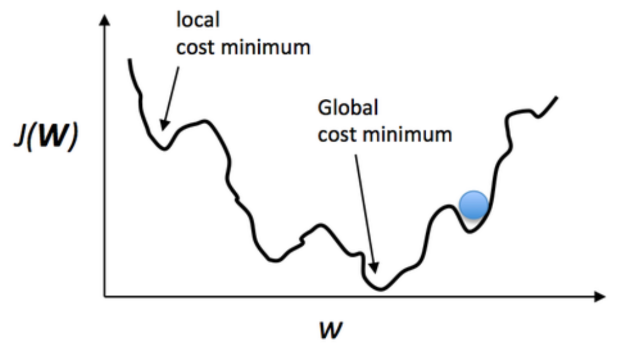
Showing the error surface with multiple minima
Momentum is an optimisation technique that helps accelerate gradient descent. It does this by adding a fraction of the previous update to the current one, which helps smooth out the path and avoid local minima.
Where:
- is the weight update in the current iteration
- is the weight update in the previous iteration
- is the momentum term (typically between 0.5 and 0.9)
Benefits of momentum:
- Helps the network "roll over" small local minima
- Speeds up learning in flat regions of the error surface
- Dampens oscillations in steep regions
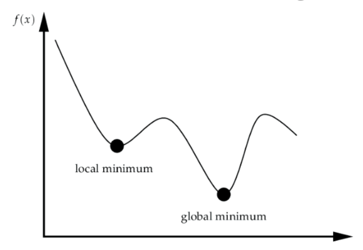
Rolling over local minima by building momentum
Function Approximation
Neural networks excel at function approximation. They can learn to approximate complex, nonlinear relationships between inputs and outputs.
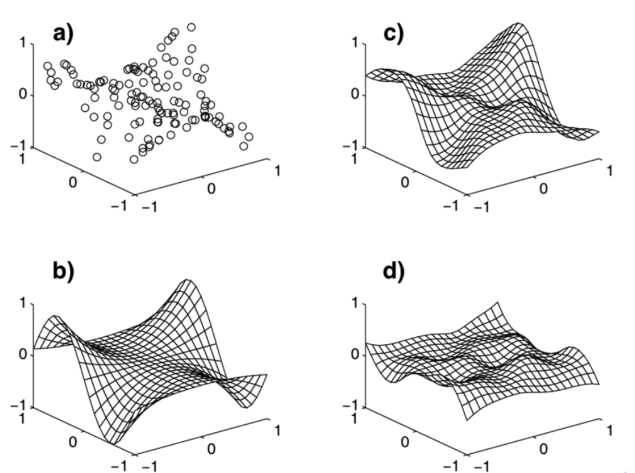
The diagram illustrates: a. Original learning samples b. The actual function that generated the samples c. The approximation learned by the network d. The error in the approximation
Practical Implementation Considerations
When implementing a neural network, several design decisions must be made:
Input and output encoding:
- How to represent categorical variables
- Whether to normalize or standardize numeric inputs
- How to encode desired outputs
Network structure:
- Number of hidden layers
- Number of nodes in each hidden layer
Learning parameters:
- Learning rate ()
- Momentum ()
- Weight initialization strategy
Stopping criteria:
- Maximum number of epochs
- Error threshold
- Early stopping using validation data
Weight initialization:
- Small random values (typically between -0.5 and 0.5)
- More sophisticated methods for deep networks
4.5 Epochs, Batches, and Iterations
Neural network training involves several key concepts related to how data is processed during training:
Epoch: One complete pass through the entire training dataset. During an epoch, every example in the training dataset is used once to update the network weights.
Batch: A subset of the training dataset used in a single update of the network weights. Batches are used when the entire dataset is too large to process at once due to memory limitations or computational efficiency.
Iteration: The number of batches needed to complete one epoch. For example, if you have 10,000 training examples and use a batch size of 200, it will take 50 iterations to complete one epoch.
The relationship between these terms can be expressed as:
Training Approaches
There are different approaches to updating weights during training:
Batch Gradient Descent: Update weights after seeing all training examples (one update per epoch).
- Advantages: More stable gradient estimates, potentially faster convergence
- Disadvantages: Requires more memory, can be computationally inefficient for large datasets
Stochastic Gradient Descent (SGD): Update weights after each individual training example.
- Advantages: Faster updates, can escape local minima more easily, works well with large datasets
- Disadvantages: Noisy updates, may not converge
Mini-batch Gradient Descent: Update weights after processing a small batch of examples (a compromise between batch and stochastic approaches).
- Advantages: More stable than SGD, more efficient than batch gradient descent
- Disadvantages: Requires tuning of the batch size
5. Preventing Overfitting
5.1 Generalisation Techniques
Overfitting occurs when a neural network performs very well on training data but fails to generalize to new, unseen data. This happens when the network memorizes the training examples rather than learning the underlying patterns.

Generalisation accuracy measures how well the network performs on data outside the training set. Poor generalisation is one of the most common problems in neural network training.
Validation Set Approach
One of the most effective methods to monitor and improve generalisation is to use a validation dataset:
Divide available data into three sets:
- Training set: Used to update weights during learning
- Validation set: Used to evaluate performance during training
- Test set: Used only for final evaluation
During training:
- Train the network on the training data, adjusting weights to reduce error
- Periodically evaluate performance on the validation set
- Save the weights that perform best on the validation set
At the end of training:
- Return the set of weights that performed best on the validation set, not necessarily those that performed best on the training set
The validation approach works because a network that has started to overfit will show increasing error on the validation set, even as its error on the training set continues to decrease.
Weight Decay
Weight decay is a regularization technique that helps prevent overfitting by penalizing large weights:
Where:
- is the weight decay parameter (typically a small value like 0.0001)
- The term gradually reduces the magnitude of weights during training
Benefits of weight decay:
- Forces the network to focus on the most important features
- Makes the network more robust to noise in the training data
- Results in smoother decision boundaries
Example: If a weight is 0.5 and with a learning rate of 0.1:
- Without weight decay:
- With weight decay:
The weight decay term subtracts a small fraction of the weight in each update, preventing weights from growing too large.
5.2 Early Stopping
Early stopping is a simple yet effective technique to prevent overfitting in neural networks.
Procedure:
- Monitor the error on the validation set after each epoch
- Stop training when the validation error:
- Stops decreasing
- Increases for several consecutive epochs
- Remains above its minimum value for a specified number of epochs
{{DIAGRAM: neural_networks.pdf, page 71, showing early stopping based on validation error}}
Early stopping criterias:
- Patience: Stop training if the validation error hasn't improved for N epochs
- Delta: Define improvement as a decrease in validation error of at least Δ
- Threshold: Stop when validation error is below a pre-defined threshold
Benefits of early stopping:
- Simplicity: Easy to implement and understand
- Effectiveness: Works well in practice for many different network architectures
- Efficiency: Saves computation time by avoiding unnecessary training
- Preserves generalization: Prevents the network from overfitting by stopping training at an optimal point
Example: If training a neural network and tracking validation error by epoch:
- Epoch 10: Validation error = 0.25
- Epoch 11: Validation error = 0.23
- Epoch 12: Validation error = 0.22
- Epoch 13: Validation error = 0.22
- Epoch 14: Validation error = 0.23
- Epoch 15: Validation error = 0.24
- Epoch 16: Validation error = 0.26
With a patience of 3 epochs, training would stop after epoch 16, and the weights from epoch 12 would be used since they produced the lowest validation error.
5.3 Network Structure Modifications
The structure of a neural network significantly impacts its tendency to overfit. Several approaches can be used to modify network structure to reduce overfitting:
Limiting Network Complexity
Limiting the number of hidden nodes or connections reduces the network's capacity to memorize the training data:
- Fewer hidden units means fewer parameters to fit
- Simpler networks tend to generalize better
- The optimal number of hidden units depends on:
- Complexity of the underlying problem
- Amount of training data available
- Noise level in the data
Dynamic Structure Modification
Instead of starting with a fixed network structure, some approaches dynamically modify the network structure during training:
Growing approach:
- Start with a simple network (few or no hidden nodes)
- Gradually add nodes as training progresses
- Stop adding nodes when performance on validation data stops improving
Pruning approach:
- Start with a larger network than necessary
- Identify and remove connections or nodes that contribute little to the network's performance
- Retrain the network after pruning
Dynamically modifying the structure can help find the optimal network complexity automatically, reducing the need for manual tuning.
Ensemble Methods
Ensemble methods combine multiple neural networks to improve generalisation:
- Train multiple networks with different:
- Initial weights
- Architectures
- Subsets of the training data
- Combine their predictions (through averaging or voting)
Ensembles tend to generalize better than individual networks because different networks make different errors, which can cancel out when combined.
Training Tips for Better Generalisation
- Rescale inputs and outputs to be in the range 0 to 1 or -1 to 1
- Initialize weights to very small random values
- Use appropriate learning rates (smaller learning rates often generalize better)
- Apply regularization techniques such as weight decay
- Consider the noise level in your training data (neural networks are quite robust to noise)
When to consider neural networks:
- Input is high-dimensional discrete or real-valued
- Output is discrete, real-valued, or a vector of values
- Form of target function is unknown
- Long training times are acceptable (since evaluation is fast)
- Human readability of the result is not important
By carefully considering these aspects of network design and training, you can significantly improve the generalisation ability of your neural networks and reduce the risk of overfitting.
6. Advanced Neural Networks
6.1 Deep Neural Networks
Deep neural networks (or deep learning) refers to neural networks with many layers. These networks have gained tremendous popularity in recent years due to their exceptional performance on complex tasks.
Deep learning differs from traditional neural networks primarily in scale and complexity:
- Many more layers (often dozens or hundreds)
- More neurons per layer
- More complex architectures optimized for specific tasks
The rise of deep learning has been enabled by:
- Increased computational power (especially GPUs)
- Larger datasets
- Novel architectural improvements
- New training techniques
However, deep networks introduce several challenges that aren't as pronounced in shallow networks:
- Overfitting becomes more likely due to the increased number of parameters
- Training difficulties due to complex error surfaces with many local minima
- Computational demands requiring specialized hardware
- Gradient-related problems including vanishing and exploding gradients
Deep neural networks have transformed many fields including:
- Computer vision
- Natural language processing
- Speech recognition
- Game playing
- Scientific discovery
These networks excel at problems where:
- There is abundant data
- The underlying patterns are complex
- Traditional algorithms struggle to capture the relationships
The true power of deep learning comes from its ability to learn hierarchical representations: early layers learn simple features, while deeper layers combine these into increasingly complex and abstract concepts.
6.2 Vanishing Gradient Problem
The vanishing gradient problem is one of the primary challenges in training deep neural networks, particularly those using sigmoid or tanh activation functions.
Cause of Vanishing Gradients
When using the chain rule during backpropagation, derivatives are multiplied together as we move backward through the network:
With sigmoid activation functions:
- The derivative has a maximum value of 0.25 (when )
- As the number of layers increases, we multiply more terms that are ≤ 0.25
- This causes the gradient to become extremely small (vanish) for earlier layers
Example of vanishing gradient: If we have 10 hidden layers using sigmoid activation:
- Each with a maximum derivative of 0.25
- The gradient contribution could be as small as
- This makes learning in early layers extremely slow or impossible
Solutions to the Vanishing Gradient Problem
ReLU (Rectified Linear Unit) activation function:
- The derivative is 1 for all positive inputs (doesn't shrink the gradient)
- Simple to compute, making it efficient
- Has become the default activation function for many deep networks
Alternative network architectures:
- Residual networks (ResNets) use skip connections to allow gradients to flow more easily
- Highway networks use gating mechanisms to control information flow
Careful weight initialization to prevent gradients from becoming too small initially
Batch normalization to keep activations in ranges where their derivatives are larger
6.3 Convolutional Neural Networks (CNN)
Convolutional Neural Networks (CNNs) are specialized neural networks designed primarily for processing grid-like data, such as images. They have revolutionized computer vision tasks.
Motivation for CNNs
Traditional fully-connected neural networks have limitations when working with images:
- Converting a 2D image to a 1D vector loses spatial information
- The number of parameters becomes unmanageable with high-resolution images
- They don't naturally capture the local patterns present in images
CNNs address these issues by leveraging three key ideas:
- Local receptive fields
- Each neuron connects to a small region of the input
- Shared weights
- The same filter is applied across the entire input
- Spatial subsampling
- Reducing the dimensionality while preserving important features
CNN Architecture
A typical CNN consists of several types of layers:
Convolutional layers:
- Apply filters (kernels) across the input to detect features
- Each filter produces a feature map highlighting areas where that feature is present
- Parameters: filter size, number of filters, stride (step size)
{{DIAGRAM: neural_networks.pdf, page 82-83, showing the convolution operation}}
Pooling layers:
- Reduce the spatial dimensions of feature maps
- Common methods: max pooling (taking maximum value in each region) or average pooling
- Help achieve translation invariance and reduce computation
Fully-connected layers:
- Usually at the end of the network
- Connect to all neurons in the previous layer
- Perform classification based on features extracted by earlier layers
Example of convolution calculations:
For an image of size 7×7 and a 3×3 filter:
- With stride 1: Resulting feature map size is 5×5
- With stride 2: Resulting feature map size is 3×3
The feature map dimension can be calculated as:
Where:
- is the input dimension
- is the filter size
- is the padding (adding zeros around the border)
- is the stride
CNNs have been remarkably successful for:
- Image classification
- Object detection
- Facial recognition
- Medical image analysis
6.4 Recurrent Neural Networks (RNN)
Recurrent Neural Networks (RNNs) are specialized neural networks designed for sequential data, where the order of inputs matters. They're particularly well-suited for:
- Time series data
- Text processing
- Speech recognition
- Music generation
- Video analysis
RNN Architecture
Unlike feedforward networks, RNNs have connections that form cycles, allowing information to persist:
- They maintain a "state vector" or "hidden state" that contains information about previous inputs
- Each step in the sequence updates this state based on the current input and previous state
- This creates an implicit "memory" of previous inputs
Mathematically, at each time step :
Where:
- is the input at time
- is the hidden state at time
- is the output at time
- terms are weight matrices
- terms are bias vectors
- is an activation function
{{DIAGRAM: neural_networks.pdf, page 84, showing RNN structure and unfolding}}
An RNN can be "unfolded" in time to appear like a deep feedforward network with shared weights across layers. This perspective helps understand both the power and challenges of RNNs.
RNN Variations
Standard RNNs suffer from the vanishing gradient problem, making it difficult to capture long-term dependencies. Two main variations address this:
Long Short-Term Memory (LSTM) units:
- Use a more complex architecture with "gates" that control information flow
- An input gate determines what new information to store
- A forget gate determines what information to discard
- An output gate determines what information to output
- These mechanisms allow LSTMs to maintain information over many time steps
Gated Recurrent Unit (GRU):
- A simplified version of LSTM with fewer parameters
- Combines the input and forget gates into a single "update gate"
- Generally performs similarly to LSTM but is more computationally efficient
RNN Applications
RNNs can be configured in different ways depending on the task:
- Sequence input to single output (e.g., sentiment analysis)
- Single input to sequence output (e.g., image captioning)
- Sequence input to sequence output (e.g., machine translation)
- Synchronized sequence input and output (e.g., video classification frame by frame)
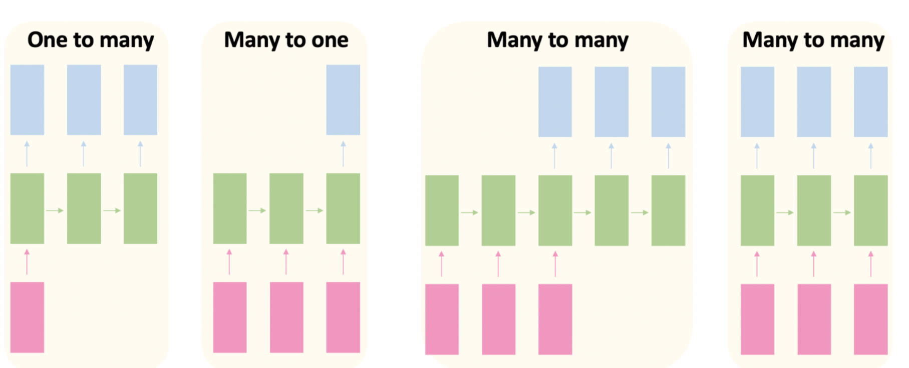
Showing different RNN configurations
6.5 ChatGPT and Large Language Models
Large Language Models (LLMs) represent some of the most advanced applications of neural networks, with ChatGPT being a prominent example. These models are based on the Transformer architecture, which has largely superseded RNNs for many language tasks.
Evolution of Language Models
Language models have grown dramatically in size and capability:
- BERT-large (2018): 340 million parameters
- GPT-2 (2018): 110 million parameters
- GPT-2 XL (2019): 1.5 billion parameters
- GPT-3 (2020): 175 billion parameters
- GPT-4 (2023): Estimated ~1 trillion parameters
This growth in model size has led to remarkable improvements in language understanding and generation capabilities.
Transformer Architecture
Unlike RNNs, Transformers process entire sequences at once using an attention mechanism:
- Self-attention allows the model to weigh the importance of different words in a sequence
- Positional encoding preserves information about word order
- Parallel processing enables much faster training than RNNs
Transformers typically use an encoder-decoder architecture:
- The encoder processes the input sequence
- The decoder generates the output sequence